Demand forecasting pipeline
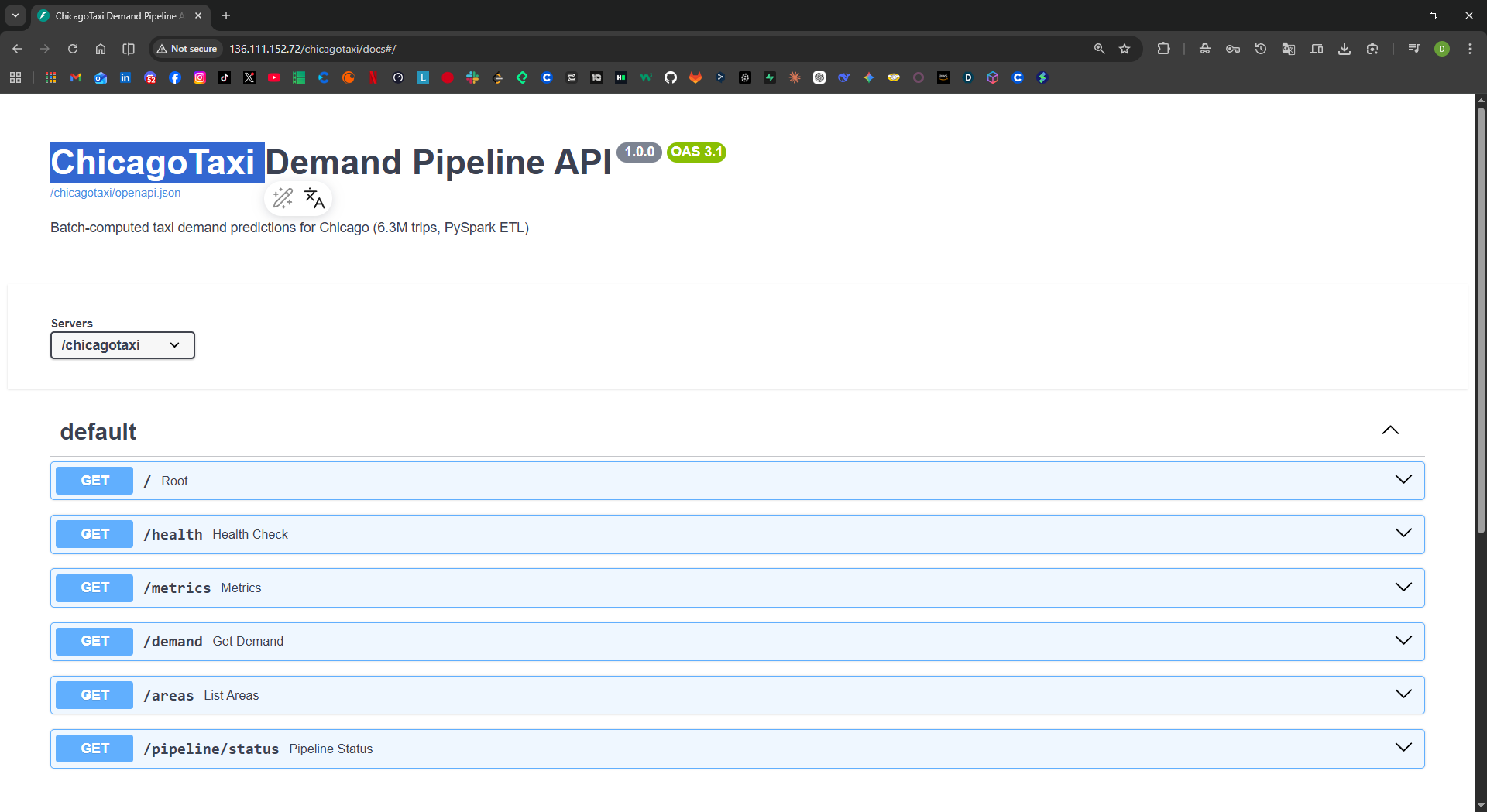
ChicagoTaxi Demand Pipeline
Process 6.3 million taxi trips into hourly demand predictions — the data engineering complement to the portfolio's online inference services.
The Problem
Chicago has 77 community areas, each with different taxi demand patterns by hour, day, and season. Predicting hourly demand per area enables driver allocation optimization. The dataset is 2.8 GB (too large for pandas), requiring distributed processing.
Business Translation
Problem
Demand changes by place and time
Driver allocation needs area/hour forecasts, not a single city-wide demand number.
Decision
Separate ETL from serving
PySpark handles heavy historical processing; FastAPI serves precomputed predictions so requests stay lightweight.
Impact
Large data becomes usable
Millions of raw trips become compact hourly demand records that can support planning or downstream dashboards.
Trade-off
Batch realism over live inference
The API avoids request-time model inference because this workload is better served as a scheduled batch prediction problem.
Architecture
flowchart LR
    subgraph ETL ["PySpark ETL"]
        A[6.3M Raw Trips\n2.8 GB CSV] --> B[Schema Enforcement\n+ Cleaning]
        B --> C[5.3M Clean Rows]
        C --> D[GroupBy\narea × hour × day]
        D --> E[357K Hourly\nDemand Records]
    end
    subgraph ML ["Training"]
        E --> F[Lag Features\nleak-free]
        F --> G[RandomForest\ntemporal split]
        G --> H[R² 0.96\nRMSE 7.87]
    end
    subgraph Serve ["Serving"]
        H --> I[Dask Batch\n19K rows/sec]
        I --> J[Pre-computed\nPredictions]
        J --> K[FastAPI\n/demand /areas]
    end
Why PySpark + Dask
| Stage | Tool | Reason |
|---|---|---|
| ETL | PySpark | Schema enforcement, distributed cleaning, partitioned Parquet export |
| Aggregation | PySpark | GroupBy over 5.3M rows into 357K hourly demand records |
| Batch Predict | Dask | Parallel inference across 4 partitions (19K rows/sec) |
| Serving | FastAPI | Query pre-computed predictions by area/hour |
pandas would OOM on the full CSV. PySpark handles the heavy ETL; Dask handles the embarrassingly parallel batch prediction. FastAPI serves the pre-computed results — no model inference at request time.
Engineering Trade-Off
Chosen: PySpark ETL, Dask batch prediction and FastAPI lookup serving. Rejected: forcing online model inference into a demand pipeline where precomputed forecasts are simpler, cheaper and easier to operate.
The reliability mindset is the same as in the BankChurn debugging deep dive: match the serving pattern to the workload instead of using one architecture everywhere.
Code Review Shortcuts
Pipeline Metrics
| Metric | Value | Context |
|---|---|---|
| Raw rows | 6,364,313 | Chicago Open Data Portal, 2013–2023 |
| Clean rows | 5,369,172 | 15.6% dropped (invalid duration, distance, area) |
| Hourly demand rows | 357,055 | Aggregated by area × hour × day |
| CSV → Parquet | 2.8 GB → 95 MB | 97% compression via columnar + snappy |
| ETL throughput | 4,741 rows/sec | PySpark local[*], 4g driver memory |
| Model R² | 0.9649 | RandomForest with lag features, temporal split |
| RMSE | 7.87 trips | On hourly demand counts |
| Batch prediction | 19,061 rows/sec | Dask, 4 partitions |
Why R² 0.96 Is Strong
This is a regression problem on aggregated hourly counts. R² 0.9649 means 96.5% of demand variance is explained by temporal + spatial lag features alone — without weather, events, or holiday calendars. RMSE of 7.87 on hourly counts means predictions are off by ~8 trips per hour per area on average. The model benefits from strong temporal periodicity and leak-free lag features (historical counts only).
Operational
| Metric | Value |
|---|---|
| Test Coverage | 91% (122 tests) |
| CI Threshold | 85% |
| Docker Image | 154 MB (chicagotaxi:v3.6.0, python:3.11-slim-bookworm) |
| Model Size | ~2 MB (RandomForest, joblib) |
| P50 Latency | 100ms /demand, 130ms /areas (GCP); 120ms / 130ms (AWS) — through ingress |
| API Endpoints | /demand, /areas, /pipeline/status, /health, /metrics |
Data Cleaning Rules
| Rule | Threshold | Rows Affected |
|---|---|---|
| Trip duration | 60s < t < 86,400s | ~8% |
| Trip distance | 0.1 ≤ d ≤ 500 miles | ~3% |
| Community area | 1 ≤ area ≤ 77 | ~4% |
| Fare range | $0 ≤ fare ≤ $10,000 | <1% |
| Comma stripping | "1,326" → 1326 |
All numeric fields |
Live Prediction
| Swagger UI | Demand Prediction |
|---|---|
 |
 |
Try It
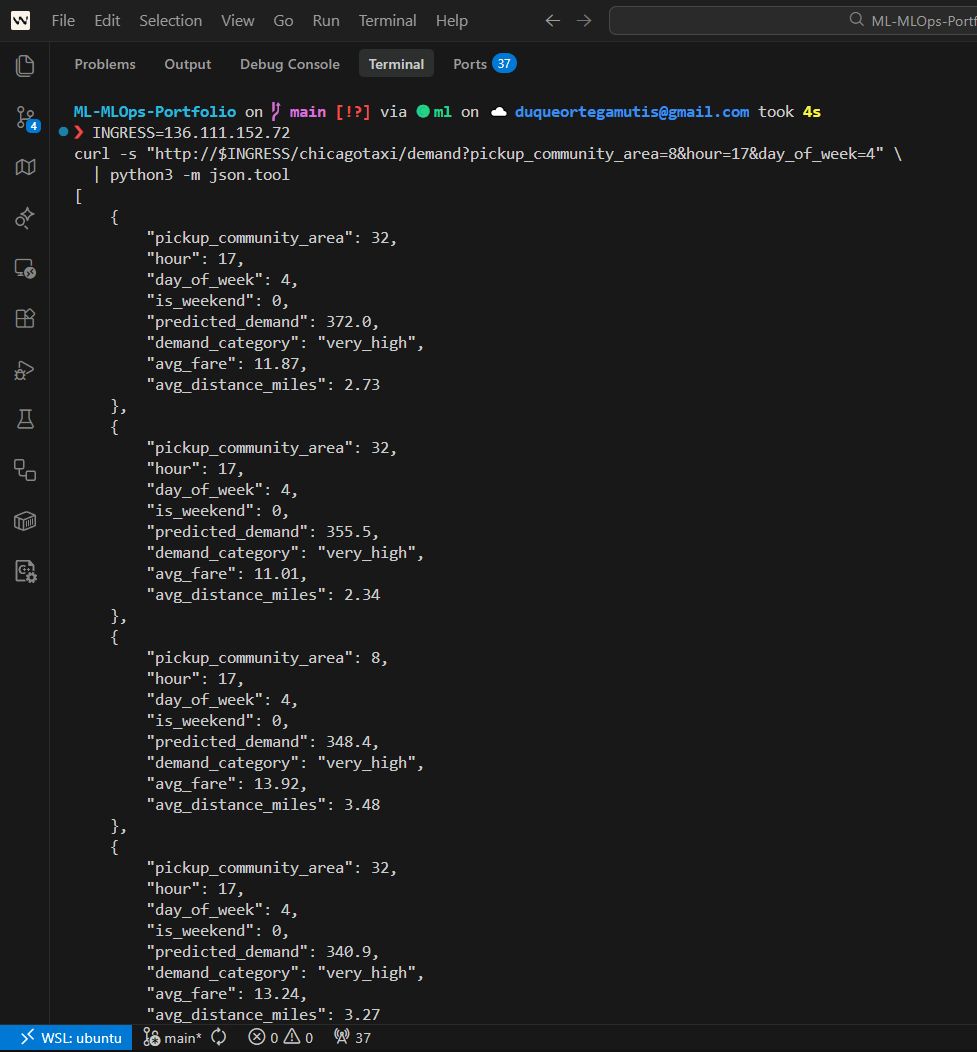
curl -s "http://localhost:8004/demand?area=8&hour=17&day_of_week=4&limit=5" \
  | python3 -m json.tool
Expected: Predicted trips for Loop area (#8) at 5pm on Friday — peak demand window.
Expected: All 77 community areas ranked by total predicted demand.
Expected: ETL metadata — rows processed, model version, last prediction batch timestamp.
Related Operating Evidence
Source: Chicago Data Portal — Taxi Trips